Handling Nonlinearities with Gurobi 12

Gurobi Summit EMEAI 2024
The Decision Intelligence Summit
https://gurobi.github.io/slides/

Pierre Bonami

Senior Developer

Agenda

Introduction
Mixed-Integer Convex Quadratic Optimization
Nonconvex Quadratic Optimization
Mixed-Integer Nonlinear Optimization

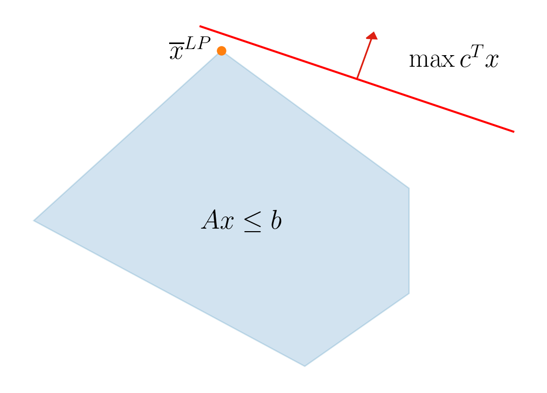
LP and MIP

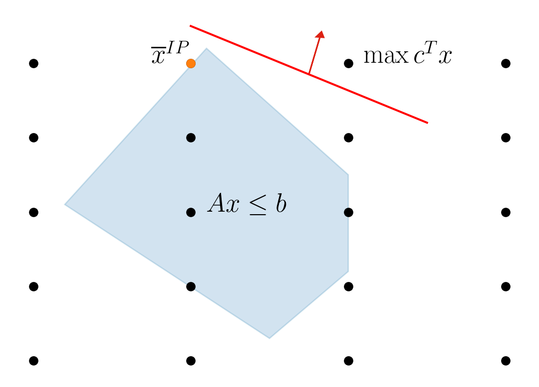
Base problems that Gurobi solves
Simplex and Barrier algorithms for LP
Branch-and-cut for MIP

Nonlinearities

Application	Phenomenon	Nonlinearity
Finance	risk	quadratic (convex)
Truss topology	physical forces	quadratic (convex)
Pooling (petrochemical, mining, agriculture)	mixing products	quadratic nonconvex
electricity distribution (ACOPF)	Alternative Current	\(\sin\) and \(\cos\) (can be made quadratic)
machine learning	—	logistic function, \(\tanh\)
chemical engineering	chemical reactions	anything

many more…

The MINLP Goal

Ideally, we seek to solve \[ \begin{aligned} & \min f(x)\\ & \text{s.t:}\\ & g_i(x) \le 0, i = 1,\ldots, m \\ & x_j \in \mathbb Z, j \in \mathcal I\\ & l \le x \le u \end{aligned} \]

\(f: \mathbb R^n \rightarrow \mathbb R\), \(g_i: \mathbb R^n \rightarrow \mathbb R\), reasonably smooth
If \(l\) or \(u\) is not finite: undecidable in general
Even assuming finiteness it’s very difficult in theory and practice
Note that integer variables are “not convex” and can be represented as a polynomial if bounded

Convex or Not Convex?

Any segment connecting two points inside the region is inside the region.

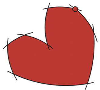
There exists two points in the region the segment connecting them is not completely in the region.

Why?

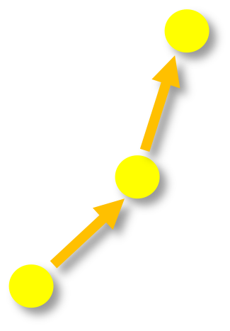
Optimization “easy” (usually)
- Start from any point in the region
- Take steps inside the region improving objective
- When there is no more step global optimum
Interior point methods for any closed convex region
Simplex algorithm for polyhedra

Optimization “hard”
- Start from any point in the region
- Take steps inside the region improving objective
- When there is no more step local optimum is reached
Need a divide-and-conquer algorithm to find a global optimum.

Nonlinearities in Gurobi

Convex

Quadratic objective: \(\min c^T x + x^T Q x\) with \(Q \succeq 0\)
Quadratic constraints: \(a^T x + x^T Q x \le b\) describing a convex region
- \(Q \succeq 0\) is a simple case, can be more complex

Nonconvex

Discrete objects: integer variables, SOS constraints
Bilinear terms: \(z_{ij} = x_i x_j\)
- Nonconvex quadratic forms: \(a^T x + x^T Q x \le b\)
Univariate functions: \(\exp\), \(\log\), \(\cos\),
- Treated directly starting with 11 (reformulated as PWL in Gurobi 9 and 10)
Nonlinear functions (closed form):
- \(y = f(x), \, x \in \mathbb R^n\)

New in Gurobi 12

Mixed-Integer Convex Quadratic Optimization

Introduction
Mixed-Integer Convex Quadratic Optimization
Nonconvex Quadratic Optimization
Mixed-Integer Nonlinear Optimization

Problem Definition

\[ \begin{aligned} & \min c^T x + x^T Q^0 x\\ & \text{s.t:}\\ & {a_k}^T x + x^T Q^k x \le b_k, k = 1,\ldots, m\\ & x_j \in \mathbb Z, j \in \mathcal I\\ & l \le x \le u \end{aligned} \]

\(Q^0, Q^1,\ldots, Q^m\) are assumed to be symmetric
- \(Q^0\) is positive semi definite
- The quadratic forms \(a_k^T + x^T Q^k x - b_k\) are second order cone representable.

The Second Order Cone

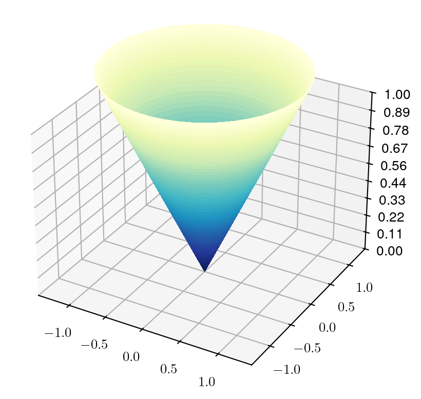
\(\mathcal L^n = \{x \in \mathbb R^{n+1}: \sum_{j=1}^n x_j^2 \le x_0^2, x_0 \ge 0 \}\)

Through simple algebra, can be represented as SOC:

\(\sum_{i=1}^n x_i^2 \le x_0^2\), with \(x_0\ge 0\)
\(\sum_{i=2}^n x_i^2 \le x_0 x_1\), with \(x_0, x_1 \ge 0\) (rotated SOC)
\(a^T x + x^T Q x \le b\), with \(Q \succeq 0\)
\(x^T Q x \le y^2\), with \(Q \succeq 0, y \ge 0\)

Very powerful but modeling sometimes far from obvious.

Not all forms recognized by solvers

Note

Our barrier algorithm needs everything converted
to SOC or linear by presolve.

New in Gurobi 12

Barrier implicitly handles bounds on variables

The Basic Branch-and-Bound Algorithm

flowchart TD
  A((c* = 0.5,  <br> x*=0.3))
  A -- "x ≤ 0" --> B((c* = 0.6,  <br> z*=2.2))
  A -->|"x ≥ 1"| C((c* = 0.8,  <br> y*=1.6))
  B -->|"z ≤ 2"| D((c* = 2))
  B -->|"z ≥ 3"| E(("c* = +∞"))
  C -->|"y ≤ 1"| F((c* = 2.1))
  C -->|"y ≥ 2"| G((c* = 1.3 <br> t* = 0.5))
  G -->|"t ≤ 0"| H((c* = ?))
  G -->|"t ≥ 1"| I((c* = ?))

  class A branchnode
  class B branchnode
  class C branchnode
  class D intfeasnode
  class E prunenode
  class F prunenode
  class G branchnode

  classDef intfeasnode stroke:#0f0
  classDef prunenode stroke:#f00
  classDef branchnode stroke:#00f

At each node of the tree:

flowchart TD
A[Solve continuous relaxation]
A --> B[Integer feasible?]
B -- no --> C[Branch]
B -- yes -->F[New solution? <br> Update best known]

In MILP and MIQP continuous relaxation usually solved by simplex.

In MISOCP/MIQCP, continuous relaxation solved by barrier.

The Outer Approximation Cut

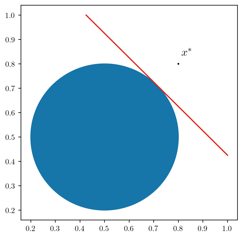
Let \(C = \{g(x) \le b: x \in R^n\}\), with \(g\) a convex function
For any \(x^* \in \mathbb R^n\), the constraint: \[\nabla g(x^*) (x - x^*) + g(x^*) \le 0 \] is valid
If \(x^* \not \in C\), it cuts \(x^*\): \[ \nabla g(x^*) (x^* - x^*) + g(x^*) > 0 \]

Outer Approximation Branch-and-Cut

flowchart TD
  A((c* = 0.5,  <br> x*=0.3))
  A -- "x ≤ 0" --> B((c* = 0.6,  <br> z*=2.2))
  A -->|"x ≥ 1"| C((c* = ?))
  B -->|"z ≤ 2"| D((c* = 2 <br> SOCP?))
  B -->|"z ≥ 3"| E((c* = ?))
  D -.-> H((c* = ?))
  D -.-> I((c* = ?))

  class A branchnode
  class B branchnode
  class D intfeasnode

  classDef intfeasnode stroke:#0f0
  classDef prunenode stroke:#f00
  classDef branchnode stroke:#00f

Drop quadratic constraints and solve an LP relaxation at each node.

Integer feasible nodes are not necessarily solutions.

flowchart TD
A[Solve LP relaxation]
A --> B[Integer feasible?]
B -- no --> C[Branch]
B -- yes --> D[SOCP Feasible?]
D -- yes -->F[New solution? <br> Update best known]
D -- no -->E[Generate OA cuts]

E --> A

Cone Disaggregation and Outer Approximation

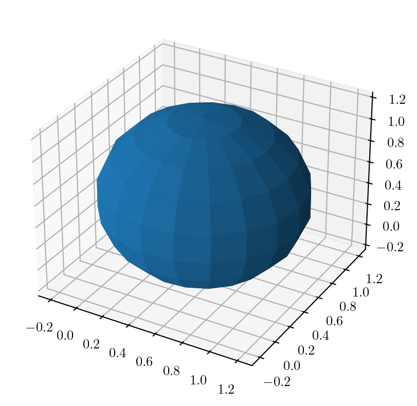
An exponential number of cutting planes is needed to approximate a convex quadratic form.

Cone disaggregation

From \[ \sum_{i = 1}^n x_i^2 \le x_0^2, x_0 \ge 0 \]

Create variables \(y_i \ge 0\), such that \(x_i^2 \le y_i x_0\) (rotated SOC)
Replace initial constraint with \(\sum_{i = 1}^n y_i \le x_0\)

Pitfalls of Disaggregation

\[ (A) \left\{ \begin{aligned} &\sum_{i = 1}^n x_i^2 \le x_0^2,\\ &x_0 \ge 0 \end{aligned} \right. \]

\[ (B) \left\{ \begin{aligned} & \sum_{i = 1}^n y_i \le x_0\\ & x_i^2 \le y_i x_0 & & i = 1, \ldots, n\\ & y \ge 0, x \ge 0 \end{aligned} \right. \]

The reformulation is correct: every solution of \((B)\) translates to \((A)\)
But a solution of \((B)\) with a small infeasibility can have a large one in \((A)\):
Suppose \(x_0 = 1\), \(y_i = \frac{1}{n}\) and \(x_i = \sqrt{\frac{1}{n} + \epsilon}\):
- Infeasibility in \((B)\) is \(\epsilon\)
- Infeasibility in \((A)\) is \(n \cdot \epsilon\)

Gurobi tries to deal with it but can be an issue.

Options for MISOCP/MIQCQP

MIQCPMethod

\(-1\) Automatic choice (default)
\(0\) Use QCP branch-and-bound
\(1\) Use Outer Approximation

PreMIQCPForm

\(-1\) Automatic choice (default)
\(0\) Leave the model as is (for B&B)
\(1\) Reformulate to SOC
\(2\) Reformulate to SOC and disaggregate

Nonconvex Quadratic Optimization

Introduction
Mixed-Integer Convex Quadratic Optimization
Nonconvex Quadratic Optimization
Mixed-Integer Nonlinear Optimization

Stepping Into a Nonconvex World

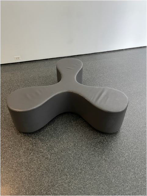
Nonconvex MIQCQP

\[ \begin{aligned} & \min c^T x + x^T Q^0 x\\ & \text{s.t:}\\ & {a_k}^T x + x^T Q^k x \le b_k, & &k = 1,\ldots, m\\ & x_j \in \mathbb Z, j \in \mathcal I\\ & l \le x \le u \end{aligned} \]

\(Q^0, Q^1,\ldots, Q^m\) are assumed to be symmetric
Continuous relaxation is NP-hard!
Solution strategy:
- Build a convex relaxation
- Refine it through branching.

Note

For simplicity sake, consider model without integer variables, in remainder.

NonConvex Parameter in Gurobi

NonConvex

\(-1\) automatic (default)
\(0\) Return error if original model has nonconvex Q objective or constraints
\(1\) Return error if presolved model has nonconvex Q that cannot be linearized
\(2\) Accept nonconvex Q by building a bilinear formulation

Since Gurobi 11

Default behavior change: \(2\) (was \(1\)).

Bilinear Formulation

For each product \(x_i x_j\)
- Introduce a new variable \(z_{ij}\)
- Add the bilinear constraint \(z_{ij} = x_i x_j\)
- Replace product with \(z_{ij}\)

\[ \begin{aligned} & \min c^T x + \left\langle Q^0, Z \right\rangle\\ & \text{s.t:}\\ & {a_k}^T x + \color{red}{\left\langle Q^k , Z \right\rangle} \le b_k, & &k = 1,\ldots, m\\ & \color{red}{Z = x x^T} \\ & l \le x \le u\\ \\ &(\left\langle Q , Z \right\rangle = \sum_i \sum_j q_{ij} z_{ij}) \end{aligned} \]

Warning

Similar to disaggregation, infeasibilities in bilinear formulation can be larger than in the original model

Bilinear Relaxation

Relax nonconvex constraint \(Z=x x^T\) using convex envelopes. \[ \begin{aligned} & \min c^T x + \left\langle Q^0, Z \right\rangle\\ & \text{s.t:}\\ & {a_k}^T x + \left\langle Q^k , Z \right\rangle \le b_k, & &k = 1,\ldots, m\\ & \color{red}{z^-(x_i, x_j) \le z_{ij} \le z^+(x_i, x_j)}\\ & \color{red}{l \le x \le u}\\ \end{aligned} \]

Convex Envelopes: Parabola

Consider the square case: \(z = x^2\)

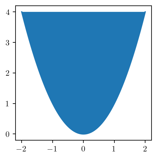
It is convex: \[ z^-(x_i, x_i) = x_i^2 \]

Can be dealt with by OA.

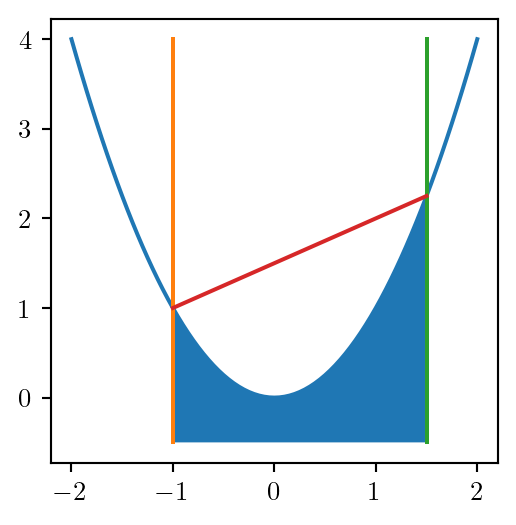
\(z^+(x_i, x_i)\) is given by the secant: \[ z^+_{ii} = (u + l) x_i - l \cdot u \]

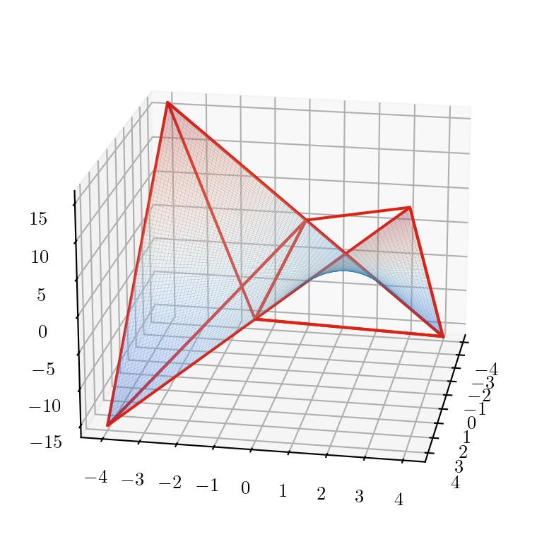
Convex Envelopes: Products (McCormick)

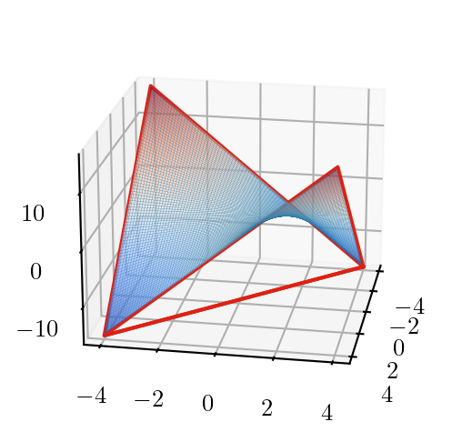
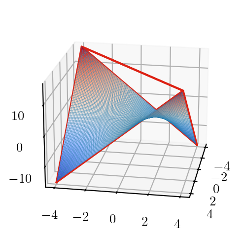
\[ z^-_{ij} = \max \left\{ \begin{aligned} & 𝑙_j x_i+ 𝑙_i 𝑥_j - 𝑙_i 𝑙_j \\ & 𝑢_j x_i + 𝑢_i x_j - u_i u_j \end{aligned} \right\} \le z_{ij} \le z^+_{ij} = \min \left\{ \begin{aligned} & 𝑙_j x_i+ u_i 𝑥_j - u_i l_j \\ & 𝑢_j x_i + l_i x_j - l_i u_j \end{aligned} \right\} \]

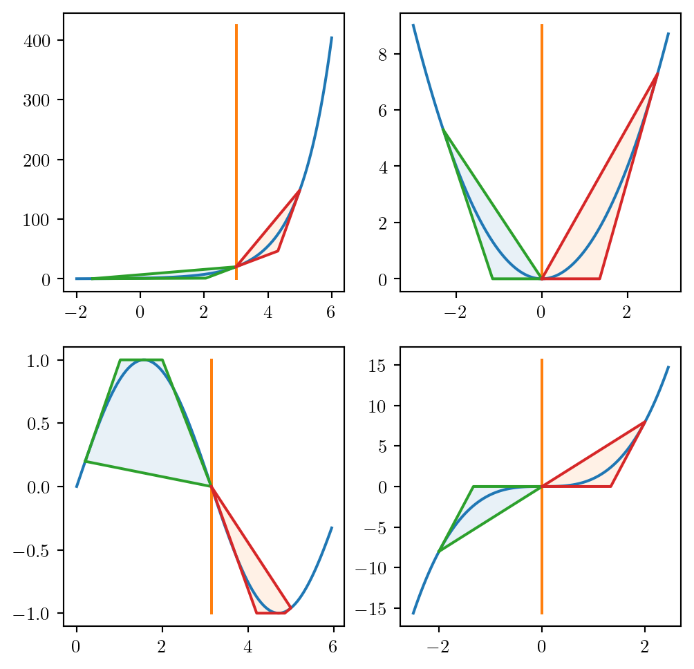
Spatial Branching

Let \((x^*, z^*)\) be the solution of the bilinear relaxation
If \(z^*_{ij} = x^*_i x^*_j\), for all bilinear terms: solution
Otherwise refine our bilinear relaxation:
- Pick \(x_i\) or \(x_j\) s.t. \(z^*_{ij} \ne x^*_i x^*_j\)
- Create two child nodes with \(x_i \le x^*_i\) and \(x_i \ge x^*_i\)
- Refine bilinear relaxation in the two nodes

Other Techniques Targeted at Nonconvex MIQCQP

RLTCuts
- Reformulation Linearization Technique (Sherali and Adams, 1990)
BQPCuts
- Facets of the Boolean Quadratic Polytope (Padberg 1989)
SDPCuts
- Relax \(Z=x x^T\) to \(Z \succeq x x^T\), and outer approximate resulting cone
OBBT:
- Optimization based bound tightening

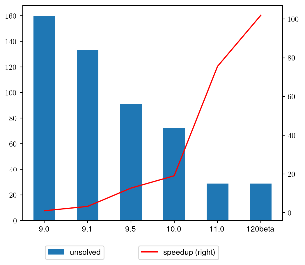
Nonconvex MIQCQP Performance History

Mixed-Integer Nonlinear Optimization

Introduction
Mixed-Integer Convex Quadratic Optimization
Nonconvex Quadratic Optimization
Mixed-Integer Nonlinear Optimization

New Nonlinear Constraints in Gurobi 12

Support for constraints \(y = f(x)\)
\(f: \mathbb R^n \rightarrow \mathbb R\)
\(y\) is a Gurobi variable, \(x\) a vector of variables

\(f\) may be composed of:
- arithmetic operations (\(+, -, \times, /\))
- a predefined list of univariate functions:
  - \(\exp\), \(\log\), \(x^a\), \(b^x\), \(\sqrt x\)
  - \(\sin\), \(\cos\), \(\tan\), \(\text{logistic}\)

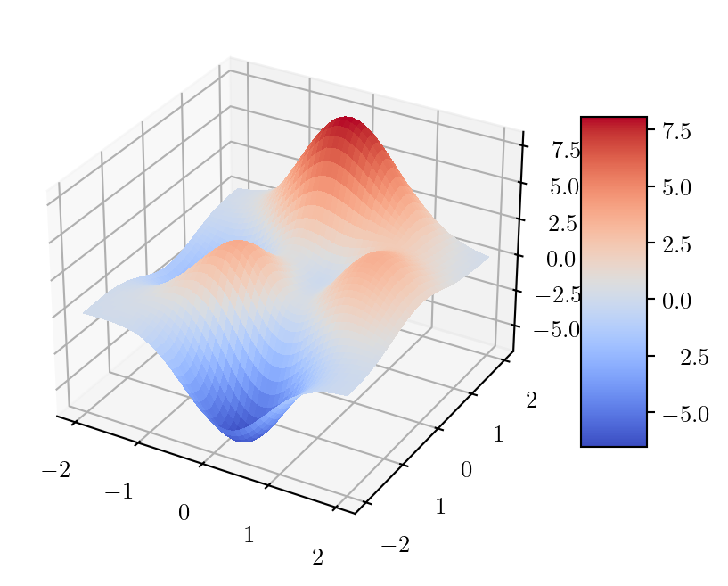
E.g. a valid function: \[ \begin{aligned} f(x) = & 3 \cdot (1-x_1)^2 \cdot \exp(-x_1^2 - (x_2+1)^2) - \\ & 10 \cdot (\frac{x_1}{5} - x_1^3 - x_2^5) \ldots \end{aligned} \]

New Python API for Nonlinear Constraints

Overloaded operators

model = gp.Model()
x = model.addVars(2, name="x")
y = model.addVar(name="y")

model.addConstr(y == x[0] * x[1] / (x[0] + 1) )

Nonlinear functions

from gurobipy import nlfunc

model.addConstr(y == nlfunc.exp(x[0]) / nlfunc.exp(x[0] + x[1]) )

Matrix friendly

X = model.addMVar((3, 3), name="X")
Y = model.addMVar((3, 3), name="Y")
Z = model.addMVar((3,), name="Z")
# follows numpy element-wise broadcasting rules
model.addConstr(Y == nlfunc.exp(X / Z))

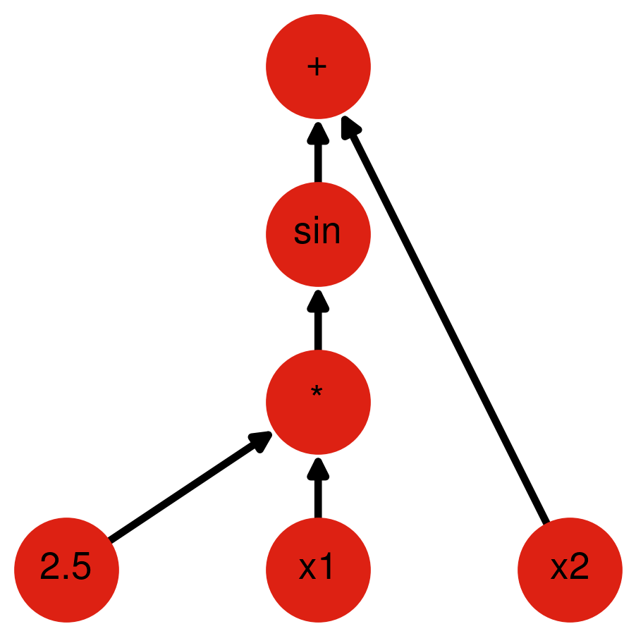
Expression Tree Representation

Internal representation of a nonlinear constraint:

Leaves: variables or constants
Internal nodes: operations on the children
Root: result of expression

index	opcode	data	parent
0	plus	-1	-1
1	sin	-1	0
2	multiply	-1	1
3	constant	2.5	2
4	variable	1	2
5	variable	2	0

Warning

In non-Python API nonlinear constraints
are entered with this representation

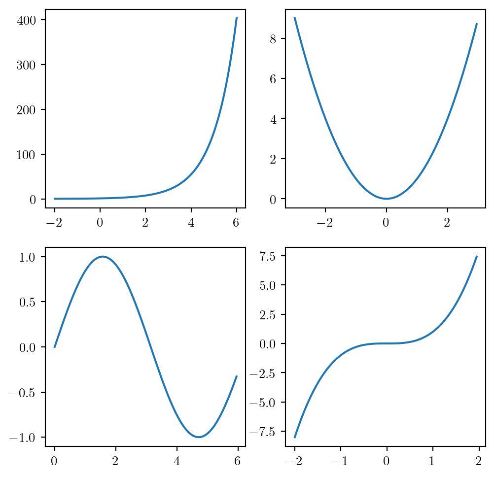
Sketch of Solution Strategy

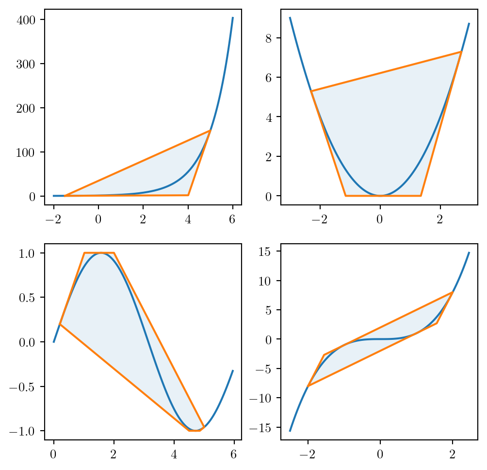
Similar to bilinear

Construct a disaggregated formulation

For each function, compute lower/upper envelope

Spatial branching to refine them

Additional difficulties:

large values (\(\exp\))
asymptotes (\(1/x\), \(\log\))
periodic functions (\(\cos\),…)

Connecting to Previous Versions of Gurobi

Since Gurobi 9.0, can state \(𝑦=𝑓(𝑥)\)

\(𝑓: \mathbb R \rightarrow \mathbb R\) is a predefined function
\(𝑦\) and \(𝑥\) are one-dimensional variables

Library of predefined functions include:

\(\exp\), \(a^x\), \(\ln\), \(\log_a\), \(\text{logistic}\)
\(\sin(x)\), \(\cos(x)\), \(\tan(x)\)
monomials \(x^a\), polynomials of one variable \(a_0 + a_1 x^1 + a_2 x^2 + ...\)

Gurobi 9 and 10: PWL approximations

Gurobi 11: Global optimization through FuncNonLinear attribute/parameter.

Comparison with Gurobi 11

Differences

Cannot use PWL for the new nonlinear functions
The list of operations in nonlinear functions slightly differs from function constraints:
- No polynomials
- No \(\log_a\) but \(\log_2\) and \(\log_{10}\)

Similarity

Disaggregated formulation for spatial branch-and-bound could be solved by Gurobi 11

Warning

In Gurobi 12 default value for FuncNonLinear attribute parameter is 1

No PWL used unless specified by the user

Example

Multinomial Regression

Adversarial Machine Learning

“Can my classifier easily be fooled?”
Basis: MNIST handwritten digit database.
Given: a (small) trained classifier and one well classified image \(\bar x\).
Goal: Construct an image \(x\) close to \(\bar x\) that is classified with a different label.

A Multinomial Logistic Regression Classifier

In this example we use multinomial logistic regression to classify digits

clf = LogisticRegression(C=50.0 / 500, penalty="l1", solver="saga", tol=0.1, random_state=4)
pipeline = make_pipeline(clf)
pipeline.fit(X, y)

Pipeline(steps=[('logisticregression',
                 LogisticRegression(C=0.1, penalty='l1', random_state=4,
                                    solver='saga', tol=0.1))])

In a Jupyter environment, please rerun this cell to show the HTML representation or trust the notebook.
On GitHub, the HTML representation is unable to render, please try loading this page with nbviewer.org.

A Training Example

\(\bar x\) is a grayscale image of \(28\times 28\) (\(=784\)) pixels
The output is a vector \(y\) of length 10 (each entry corresponding to a digit)
The image is classified according to the largest entry of \(y\)
The entries of the vector are computed using SoftMax and are probability estimates


Predicted label is 1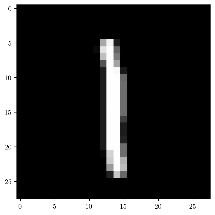

y = [0.   0.98 0.   0.   0.   0.   0.   0.   0.01 0.  ]

Multinomial Logistic Regression and SoftMax Function

The multinomial regression computes one regression vector for each label:

\[ r_l(x) = a_l^T x + b_l, \, l=0,\ldots,9 \]

Then the SoftMax function is applied to obtain the vector \(y\):

\[ y_l = g_l(x) = \frac{e^{r_l(x)}}{\sum_{k=0}^{9} e^{r_k(x)}}, \, l=0,\ldots, 9 \]

Tip

\(g\) is typically a function that is now easy to write in Gurobi 12!

A Variant of the Classical Adversarial Problem

Index \(l= 1\) of \(y\) is correct. Can we trick the classifier to classify a nearby image with index \(w= 5\)?
An image \(x\) with \(y_w > y_l\) is a counter example
Here we additionally require the probability of \(l\) to be smaller than \(0.25\)

\[\begin{alignat}{3} \max_{0 \le x \le 1, y} \quad & y_w\\ \mbox{s.t.} \quad & \|x - \bar{x}\|_1 \le \delta\\ & g(x) = y \\ & y_l \le 0.25 \end{alignat}\]

Notations

\(g\) the prediction function of the logistic regression

\(\delta\) the width of the neighbourhood

The gurobipy Model

m = gp.Model()
delta = 6
right_label = 1
wrong_label = 5

# Create input/output variables
x = m.addMVar(xbar.shape, lb=0.0, ub=1.0, name="x")
y = m.addMVar(10, lb=-np.inf, name="y")

# Constrain x to 1-norm neighbourhood around \bar x
eta = m.addMVar(xbar.shape, lb=0, ub=1, name="abs_diff")
m.addConstr(eta >= x - xbar)
m.addConstr(eta >= -x + xbar)
m.addConstr(eta.sum() <= delta);

# Upper bound on probability of right label
y[right_label].UB = 0.25

# Objective: Maximize the probablilty of wrong label
m.setObjective(y[wrong_label], gp.GRB.MAXIMIZE)

# Insert the neural network in the gurobipy model
pred_constr = gml.add_predictor_constr(m, pipeline, x, y, predict_function="predict_proba")

Solving the Model

Gurobi Optimizer version 12.0.0 build v12.0.0rc0 (mac64[arm] - Darwin 23.6.0 23H222)

CPU model: Apple M3 Pro
Thread count: 4 physical cores, 8 logical processors, using up to 8 threads

Optimize a model with 1589 rows, 1588 columns and 3940 nonzeros
Model fingerprint: 0xa32573da
Model has 20 general nonlinear constraints (20 nonlinear terms)
Variable types: 1588 continuous, 0 integer (0 binary)
Coefficient statistics:
  Matrix range     [1e+00, 1e+00]
  Objective range  [1e+00, 1e+00]
  Bounds range     [2e-01, 1e+00]
  RHS range        [4e-03, 6e+00]
Presolve model has 20 nlconstr
Added 11 variables to disaggregate expressions.
Presolve removed 1442 rows and 966 columns
Presolve time: 0.01s
Presolved: 248 rows, 634 columns, 4960 nonzeros
Presolved model has 10 bilinear constraint(s)
Presolved model has 10 nonlinear constraint(s)
Warning: Model contains variables with very large bounds participating
         in nonlinear terms.
         Presolve was not able to compute smaller bounds for these variables.
         Consider bounding these variables or reformulating the model.


Solving non-convex MINLP

Variable types: 634 continuous, 0 integer (0 binary)

Root relaxation: objective 1.000000e+00, 282 iterations, 0.00 seconds (0.00 work units)

    Nodes    |    Current Node    |     Objective Bounds      |     Work
 Expl Unexpl |  Obj  Depth IntInf | Incumbent    BestBd   Gap | It/Node Time

     0     0    1.00000    0   20          -    1.00000      -     -    0s
     0     0    1.00000    0   16          -    1.00000      -     -    0s
     0     0    1.00000    0   14          -    1.00000      -     -    0s
     0     0    1.00000    0   14          -    1.00000      -     -    0s
     0     0    1.00000    0   14          -    1.00000      -     -    0s
H    0     0                       0.7396035    1.00000  35.2%     -    0s
     0     2    1.00000    0   14    0.73960    1.00000  35.2%     -    0s

Explored 360 nodes (3690 simplex iterations) in 0.19 seconds (0.37 work units)
Thread count was 8 (of 8 available processors)

Solution count 1: 0.739604 

Optimal solution found (tolerance 1.00e-04)
Best objective 7.396035216634e-01, best bound 7.396198121843e-01, gap 0.0022%

Solution

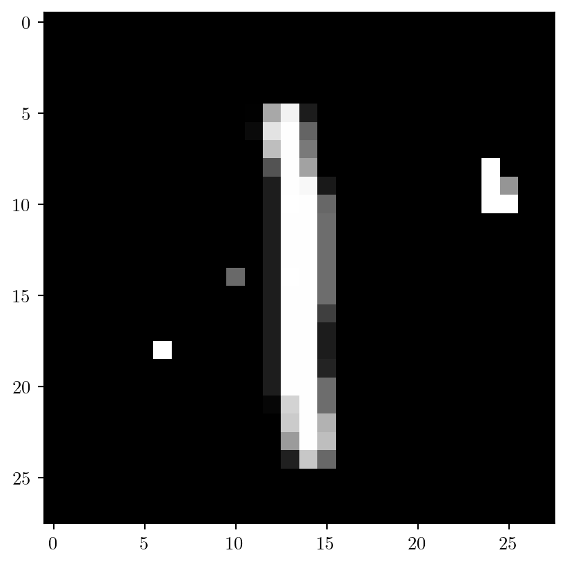
Label probabilites for perturbed image:
 [0.   0.24 0.   0.   0.   0.74 0.   0.   0.01 0.  ]

Softmax Model in Gurobi ML

# We want to write y_j = e^z_j / sum_j=1^k e^z_j
# y_j are the output variable z_j = input @ coefs + intercepts

# Store the e^z_j in a nonlinear expression
exponentials = nlfunc.exp(linear_predictor)

# The denominator is the sum over the first axis
denominator = exponentials.sum(axis=1)

# Voila!
gp_model.addConstr(
    output == exponentials / denominator[:, np.newaxis]
)

Gurobi 11 Style Model

linear_predictor_vars = gp_model.addMVar(
    output.shape, lb=-gp.GRB.INFINITY, name="linear_predictor"
)
gp_model.addConstr(linear_predictor_vars == linear_predictor, name="linreg")
predictor_model.linear_predictor = linear_predictor_vars

exponentials = gp_model.addMVar(output.shape)
exponentials = exponentials
denominator = gp_model.addMVar((output.shape[0]), lb=epsilon)

num_gc = gp_model.NumGenConstrs

for index in np.ndindex(output.shape):
    gp_model.addGenConstrExp(
        linear_predictor_vars[index],
        exponentials[index],
        name=predictor_model._indexed_name(index, "exponential"),
    )
gp_model.update()
try:
    attributes = predictor_model.attributes
except AttributeError:
    attributes = {}
for gen_constr in gp_model.getGenConstrs()[num_gc:]:
    for attr, val in attributes.items():
        gen_constr.setAttr(attr, val)
gp_model.addConstr(denominator == exponentials.sum(axis=1))

gp_model.addConstrs(
    output[i, :] * denominator[i] == exponentials[i, :]
    for i in range(output.shape[0])
)

Comparisons of Models Performance

Using Gurobi 12 beta:

PWL (à la Gurobi 10 )
Univariate (à la Gurobi 11)
Expressions (à la Gurobi 12)

		v10	v11		v12
	#models	# viol.	Speedup	# viol.	Speedup	# viol.
	50	15	19.5	0	35.2	0

Algorithmic Enhancements for Nonlinear Constraints

Presolve

Works on the full nonlinear expressions:

Propagations
Simplifications: e.g. \(0 \times f(x) \rightarrow 0\)
Reformulations: e.g. \(\sin(-x) \rightarrow -\sin(x)\), \(\exp(M) \times \exp(x) \rightarrow \exp(M + x)\)
Careful disaggregation

Branch-and-bound search

Can check original nonlinear constraints for feasibility:

Reject solutions with too high violations
May fail to reach MIP gap if a node is not solvable

flowchart TD
A[Solve relaxation]
A --> B[Feasible in <br> Disaggregated Space?]
B -- no --> C[Branch]
B -- yes --> D[Feasible for <br> original constraint?]
D -- yes -->F[New solution]
D -- no -->E[?]

linkStyle 0,2,4 stroke:#dd2113,stroke-width:4px;

A Computational Comparison of Gurobi 11 and 12 for Nonlinear Models

Consider models from public library minlplib.org

862 models that are not quadratic
Converters provided by GAMS
- V11 way: disaggregated formulations using function constraints
- V12 way: original formulation using nonlinear constraints
Keep 655 models that are not simplified to quadratic by end of presolve
The two formulations are equivalent but V11 can exploit infeasibilities

Violated Solutions

Performance

Table 1: v11 vs v12 performance

(a) Univariate

	#models	Speedup
> 0	419	1.00
> 1	178	0.98
> 10	121	0.87

(b) Univariate vs. Expressions

	#models	Speedup
> 0	422	1.30
> 1	182	1.63
> 10	127	1.69

Table 2: v11 vs v12 quality

	v11 univ	v12 univ	v12 expr
Unsolved	30	36	16
Sub-Optimal	0	0	3

Sub-Optimal terminations

Cases where cannot branch but solution still violated

Sub-optimal termination (unable to solve some node relaxations)
Best objective 7.000338563098e+00, best bound 6.998594162348e+00, gap 0.0249%

Conclusions and Outlook

(nonconvex) MIQCP solver state of the art, tremendous improvements
Second iteration of MINLP solver:
- Real nonlinear constraints
- Improved stability and performance
Current weaknesses and outlook
- Focus is on global optimality
- Nonlinear optimization capabilities for locally optimal solution
- Difficult to get high accuracy (\(< 10^{-5}\)) by branching only